English

MODELLING LAND USE DYNAMICS IN THE SPANISH NETWORK OF NATIONAL PARKS AND THEIR HINTERLAND (DUSPANAC)

Castellano

DUSPANAC GIS Documentation

Chapter 2: Creating raster land cover maps for each National Park from the corine data for all Spain

In chapter 1, 3 CORINE Land Cover maps were created for each of the 14 national park areas, by downloading the appropriate data from the website of the European Environment Agency (EEA), clipping the data, projecting as Lambert Azimuthal Equal Area. A geodetic transformation was applied to the National Park and Use and Management Plan (PRUG) boundaries, from the website of the autonomous body for national parks (OAPN), to convert them from European Datum 1950 (ED1950) to European Terrestrial Reference System 1989 (ETRS1989), LAEA projection, same as the corine datasets. In this chapter we discuss how to clip the raster data using Extract by Mask (spatial analyst tools-extraction-extract by mask) in ArcGIS, or in ArcView 3.2, with spatial analyst and grid analyst extensions (grid analyst menu-extract grid theme using polygon). The procedure was as follows:

1. Clip all raster grids to area of PRUG from from corine90, 00 and 06 (LAEA projection), in ArcView 3.2, with Extract by Mask (ArcGIS) or Extract Grid Theme (ArcView 3.2). Those parks that did not have a PRUG were given a buffer zone of 800m (by applying the buffer command to the park boundary shapefile and then clipping as per the instructions above).

2. Export to ascii format (Arc toolbox-conversion tools-raster to ASCII).

3.Convert park boundaries (Arc toolbox-conversion tools-Polygon to Raster) and export to ascii as above. Note that here, we do not need the extended study area boundaries, just the original core park study area.

4. Import to ILWIS 3.7 open (Operations toolbar-import/export-import). ILWIS can be downloaded from 52 degrees north. This version runs under windows xp and under linux with the wine compatibility layer. Also just about works in Windows 7, but is rather unstable.

5. classify maps according to appropriate corine legend as follows.

• first create a new Domain, give a name (aigcorine), and make sure the “group” box is ticked.
• fill in limit values, class names, and set the representation classes to the appropriate corine colours.
• The reclassified category map with the corine legend is created with the “slicing” command
  newaig90prug=MapSlicing(aig90prug, aigcorine)

6. For the cross tabulation analysis (below), we need, for each national park, the park study area raster map (a a binary integer map, 0 and 1), and the land use maps for corine 90, corine 00 and corine 06 that we created above in step 1 for each park, including the land use in the park hinterland zone (either the PRUG boundary or, if there wasn't a PRUG or if the PRUG is smaller than the national park study area, the 800m buffer zone). The Metronamica modelling software does not recognise null values (the '?' in ILWIS). The following steps explain how to reclassify the ILWIS raster map to remove null values, and how to ensure that the study area has the same cellsize and the same number of rows and columns as the land use maps (this can be carried out in ArcGIS beforehand, but just in case this step was omitted, its useful to know how to correct this problem).

• So, to create the binary study area map, first (if necessary) apply a resample so that the study area map has the same columns and rows as the land use maps. Here we use the data for Aigüestortes y Estany de Sant Maurici national park.
  aigpn_resamp:=MapResample (aigpn, newaig90prug.grf, BiLinear)
• Create a new map aigpn_resamp resampled to the new area of newaig90prug.
• Recalculate this map using the IFUNDEF command to remove null values (if is undefined; null). We chose values 0 (outside park limits) and 1 (inside park limits) for the new map.
  aigstudy = IFUNDEF (aigpn_resamp,0,1)

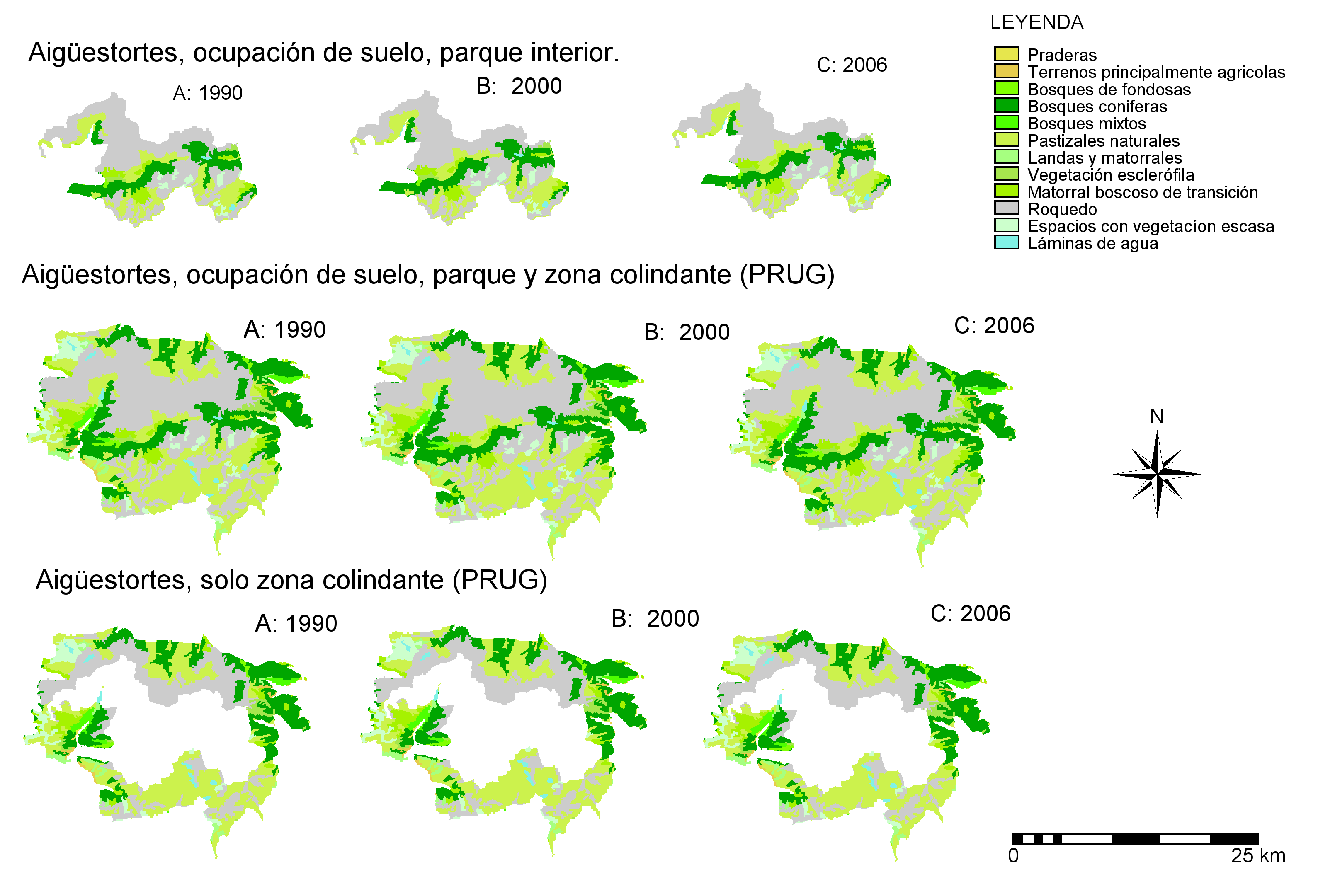
7.Now we have a park boundary study area for each park, plus our 3 land use maps for each park, including all the area within either the use and management plan (PRUG) boundary or an 800m buffer zone. Using the technique of cross tabulation analysis, we want to investigate land use changes inside the park (A), inside the whole area of the park plus the PRUG/buffer hinterland zone (B), and inside the hinterland zone only (C). To do this, we use the national park study area to "cut out" the land use contained by the study area (producing map A). The original map that we used as a template is of course map B. And the area left over after the cut-out (sometimes, in vector GIS terminology, referred to as "cookie cutter") operation, will be map C. Thus:

• newaig90park = IFF(aigstudy=1, newaig90prug,?)  [map A]
• newaig90prug = newaig90prug  [map B]
• newaig90buff = IFF(aigstudy<>1, newaig90prug,?)  [map C]

Now we just need to repeat the process for land use 2000, and land use 2006, and then carry on to do the same for all the other 14 national parks. Note that here, we use the null value symbol (?), rather than 0, as metronamica treats 0 as a land use value. There are other ways to deal with this problem that won't be discussed here. Here are the nine final land use maps for the park used in our example, Aigüestortes y Estany de Sant Maurici, prepared in ILWIS 3.7 (since there was very little change observed in this national park using corine land cover, the maps are all very similar).